A Grand Adventure - Perspectives and Projections

The past few weeks or so I've begun a conquest to teach myself OpenGL graphics programming. It occurred to me that I should probably be sharing this experience. I have a fairly limited knowledge of lower level graphics and, although I intend to change it shortly, linear algebra. I have some basic knowledge of each, but not enough to do anything all that exciting. What I intend to do with this and potential future entries is to explain the concepts of graphics programming in a more intuitive sense. I'm less worried about the mathematics behind it. Although it is incredibly important, sometimes intuition should lead to the mathematics, rather than the mathematics leading to intuition.

The first stop on this journey will try to go into some detail about the viewing plane. Since computers and other output devices are two dimensional, well, this makes it a bit of a challenge for 3D graphics. OpenGL handles a lot of the math for us. We provide the world in three dimensional coordinates, but the world is then projected onto the two dimensional screen.

First, I'd like to give a small overview on a basic and inherently intuitive concept of depth that we all share. For example, if you have two objects, and one is "in front" of the other, how would you see this in real life? Think of two tree's, one nearby and one further away. The tree further away would appear smaller then the tree in front of the other. Further, the tree closer could obstruct part of the view of the one further away. This is the magic of depth.

There are two primary modes of rendering in OpenGL that project onto the screen differently. There's orthogonal mode and perspective mode. I'll start with orthogonal since that's really what we deal with intuitively using the typical x,y plane. There are some differences, but we'll get to that.

An orthogonal projection is really a mode that lacks any real depth. While depth is present, it's not distinguished when being rendered in terms of the objects size. Still, orthogonal can give primitive versions of depth. We may still specify that an object is in front of or behind an object, but the size of the object will be the same, no matter how close or how far away. The depth and size calculations are not present here. The only thing is that one will render "over" the other object. Take the example below:

Notice how there is a small illusion of depth here. It's clear that the sore to the eye smile face is rotated about the y axis. The cubes to the right have some idea of being "behind" the ones to the left. This is an orthogonal projection. The cubes, regardless of where they are, are all the same size. The illusion of depth is not completely satisfied here. However, orthogonal projections do exist for a reason. If you want some static information displayed that isn't really part of the world, such as the health bar or other characterizations, there's no need for depth. Additionally, if we were to create a 2D game, well, orthogonal is more than satisfactory.

Now, perspective projections are a little different. Many of the mechanics are the same, but the addition is that as objects are further away, then their size is smaller. For example, you might see layers of trees on a mountain top that, as those layers get further away, they appear smaller. That's not all, however, they also appear to move slower. This effect is generally called parallax scrolling. Perspective gives us this ability with very little extra work. Lets go right to the example.

Notice how in this case, the cubes that are rotated appear smaller or larger depending on where they are in relation to the viewer. Here, the illusion of depth is more or less enhanced. Without going into a lot of extra detail, the major difference behind the scenes here is that OpenGL scales the objects further away based on the depth of an object in relation to the viewer. Of course, depth is based on the current rotation, among other things.

I've tried to keep this as intuitive as possible, and perhaps it's a little wordy, but really, the only reason I've finally managed to learn this is by doing. Anyone interested in this type of work needs to spend a healthy amount of time just playing around as I have with the above examples.

Until next time!

Solving the Knapsack Problem

So, a while back I promised that I'd go through the knapsack problem. The time is nigh!

The knapsack problem is as follows. You are trying to move the maximum number of objects as possible, but your knapsack can only carry up to a maximum weight W. This means that each object is assigned a weight.

Now, to solve this problem we need to think a little differently than we traditionally think about the more basic problems in computer science. We're left with some fairly basic assumptions from an algorithm perspective

1. An object can only be used once
2. If the weight of an object being tested exceeds the current knapsack weight, it also cannot be used
3. Order does not matter, because the objects can be used in any combination. This implies that with a brute force approach, there are n²-1, where n is equal to the total number of objects, possible combinations which can add up quite quickly with a large data set.

We can observe one additional item that can help us reduce the number of combinations. If we sort the data set before invoking the algorithm and we exceed the weight W as we sum up items to check, and we can assume that any item after that will also fail.

We will use the input list of {10, 40, 29, 4, 12, 45, 32, 34}, and W = 100 as an example for the remainder of this entry.

To begin with, we'll sort the array to {4, 10, 12, 29, 32, 34, 40, 45}. We should also note that n here is equal to 8. There are a few different ways to go about this, but one of the ideal ways is to use recursion. You can view this as a tree, or even a forest where each element in the list can act as the root node, and then traverse each path to act as the sum. This first step of thinking recursively is key in solving the problem.

For example, we'll start with 4. We'll use a depth first search method and continue along the path of the sorted list. 4 + 10 + 12 + 29 + 32 = 87. If we add 34, we get 121 which is over the weight limit of W, which in this case is equal to 100. In this example, we can also stop looking further down that side of the tree because any weight after 32 is also going to fail the test.

So we're at a point where it's not easy to visualize without an image, so I'll paste one below.

34 is the last option we try in this path. Currently, it's just a linear tree

Given this, we can see that the node of 32 gives us a maximum possible weight of 87 from this path. So we need to try other solutions. So we remove 32 from the solution, and try 34. This gives 4 + 10 + 12 + 29 + 34 = 89. Our maximum weight is now 89, and we're once again confronted with an issue where anything after 34 will fail our weight test.

So once again this pattern continues and we remove 34 from the solution and try 40. This gives 4 + 10 + 12 + 29 + 40 = 95. Now our maximum obtained weight is 95, which again makes the other solutions at this point in the algorithm incorrect. We also, once again, run into the issue of anything after 40 will fail the test, so we pop 40 off of the list and try 45.

For those paying attention, their intuition might have gone off on this part. If we add 45, we get 4 + 10 + 12 + 29 + 45 = 100 exactly. In our problem, there is no need to continue. So while this was an apparently short run, it's important to note that we made end up going through all possible combinations - the failed tests when  it reaches > 100. However, the worst case is still n² - 1 because we may have an input list that never exceeds the weight limit W. Below is a full tree of the attempts made with 4 as a starting point.

So you can see how it will begin to branch out. If we did not find 45 as a solution, we would then backtrack to 12 and start with a similar idea and begin adding each of the remaining numbers and stopping when the current weight > W.

Similarly, if, for the sake of argument, we did not find any solutions that began with 4, we would eventually pop back all values and start with 10 as the root node. This is called backtracking, and with the way the algorithm works that once something fails, we revert to an earlier state which lends itself well to recursion.

This solution however is only one way, and still runs the risk of a high number of operations and checks depending on the solution set. So we need to be a little more clever to reduce this. Recursion is also the entry way to thinking dynamically. With that, I mean there is a technique called dynamic programming. In a nutshell, dynamic programming uses stored data to prevent the recalculation of items in an algorithm. For example, if a certain maximum weight has already been calculated for a certain combination, then we can store that in an array and consult that instead of redoing the calculation. With recursion, this can make a particular difference as we'd be removing complete levels of the tree.

This is the way my group in my data structures class went about it. This not the only, or even the best solution. I'm leaving this entry intentionally brief in the description because while this is a "correct" solution, there is a more clever way to think recursively which is something I learned sometime later. In the next entry, I will go into more detail on a solution that more accurately paves the way to dynamic programming. As this solution stands, it becomes difficult to represent with a tabular approach.

Until next time!

Detour for Tetris Attack

Hello everyone. I know I promised a technical entry on AVL trees and I promise I will get to it! However, I've enjoyed some downtime the past couple weeks, and also moved onto a small side project while John tries to get the map system running as most of the stuff I need to do relies heavily on that update. So, I'll be taking a slight detour to talk about a game named Tetris Attack.

Those who know me will definitely vouch for me on this, I am extremely fond of Tetris Attack. It throws people off all the time, but this is not Tetris as most know it. For those who don't know what Tetris Attack is, I highly recommend checking it out. It's a game that came out with the Super Nintendo, which I know is old, but it's still probably my favorite game today. Here is a video showing some aspects of the game on YouTube by MarkoManX.

The beauty of this game is that it's undeniably simple when you start out. You get matches of 3 in vertical or horizontal lines to clear the blocks. In this game, diagonals do not matter. If you get more than 3, that is a combo. If you get a match, and those blocks fall and make another match, this is called a chain. Chains naturally give more rewards, particularly for longer chains. As each chain can make another match, and another, and another ... up until the skill of the player interferes or there is no possibility within the constraints of the current block set up.

So, for a long time I've wanted to build my own little clone of the game. Nothing big, but something that shows I can sit down and figure out the mechanics in a discrete way. So today, as it relates to computer science, I'm going to talk about how I figured out how to make the matching algorithm work in my prototype. Trees are not far off, as Trees can be made from the subset of a graph and is in fact a common thing to do. Particularly for minimum spanning trees which would solve the traveling businessman problem. For those that don't know the problem, it's essentially about a businessman that wants to travel to a set of cities S using the minimum possible cost or distance using the available routes between them. I do not use graphs explicitly, but thinking of the grid as a graph can help.

First, allow me to explain some of the components via visuals.

I grabbed the block images from a game called tetattds, which is another remake of the game for the Nintendo DS. I downloaded the source and looked around to give me a general idea of how they thought. Now, I promise, whatever I came up with in my code is on my own merit, as I'm pretty certain whatever is in the source for tetattds is better than mine because I really am not sure what they did in this regard. I'm just here to explain the basic, high level approach one can take, and am not advocating it as the best or only way.

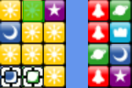
Anyway, take a second and given when you know already (3 or more blacks makes a match, anything more than 4 makes a combo, etc), what match do you think the above image will make for the yellow blocks?
..
..

This will make a 7 (seven) combo. Meaning, 7 blocks are matched. Some of you might be thinking, "But wait! There are eight yellow blocks touching!" and you would be correct. The issue is that the top left most yellow block is not in any adjacent combination of 3 or more in a row either vertically or horizontally.

So how do we account for such challenges?

The first thing to realize is that the field of play is a n x 6 grid. Such as:

[1,1][1,2]...[1,6]

[2,1][2,2]...[2,6]

...

[n,1][n,2]...[n,6]

That is, it can have infinitely many rows, but only 6 columns. There can be empty blocks as well as the normal types. We don't always want to check for a match because then it would be a waste of resources, so what we first need to think about are the conditions in which a pop might be invoked. These are a cursor swap, a falling block, or a row of blocks being raised from underneath. In each of these cases, a "NeedPop" flag is set on the individual block, and during the game loop it sweeps the field and looks for that state. If it finds it, it commences the algorithm to look for matches. This idea was brought forth by John, because originally I just called the algorithm when any of the above mentioned events occur, but this gives a degree of freedom while making some things simpler, and other things more complicated which I may get to in a future post.

Now for the interesting bit. The grid, in its form to the game, can be thought of a graph. Each block can have four connections (also called edges) to the block above, below, to the left of, and to the right of a block. The basic premise of the algorithm to detect a match is a breadth first search algorithm. For those that don't know, this is basically a mechanism for visiting the vertices in a graph (or tree) by visiting each vertex and its children before moving onto the childrens children. This is in contrast to a depth first search which will search the remaining depth of the first searched child of a node (recall what I mentioned about trees in my last post) to its height, before moving back up the tree to check other children of a node. In fact, a tree structure is represented from both the breadth first search and depth first search traversal algorithms.

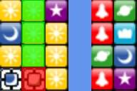
So lets do a quick run through. We'll start with the top left block, which I already mentioned did not make it in the final match, and I'll explain why in terms of the algorithm. I'll mark a node as visited by showing a transparent green box over the block.

First thing is first, we need a Queue to keep track of what blocks we're processing. So first in the Queue is the top left block. We'll mark this block as visited. Since we're concerned with the vertically and horizontally adjacent blocks, we search those and add them to the Queue if they match with the block that started with the search. So what we end up with is the below, with green marking a match and red marking a non match.

So note that we do get a same tile to the right, but it stops with the start and since the number is < 3, we don't add the matched tile to the queue, and because there's nothing below (And empty/invalid tiles to the left and above), we stop processing and move on to the next one adjacent to it (To form the sweep, but the algorithm will work from any position, and i'll demonstrate that after).

I'll take the next one step by step.

First, we take the block at row 1 (from the top), and column 1.

Then we start processing that Queue. We'll start with verticals as that's what I started with in my code. So we look down, and find that we have a matching tile, and we check below that, and we have a third matching tile so we add to the set that maintains all matching tiles, and at this point we only have the three. The algorithm will check the tile below that as well, and find that we have no matching tile (Excuse the cursor image in there, I kept it in to show that's what the cursor looked like, but there's a blue and green block with the cursor). After checking all verticals, we get the below.

In this process, we added the two below the first one to a Queue, in order. That means that we're now checking the second block. In this case, we're moving down the grid. My algorithm knows that we're going that way, so we only need to check horizontals. This means that we'll first check the left, realize there's nothing, and check to the right, add the matching block to the Queue (this is important), and find nothing so we did not find a match here, and nothing is added to the match set. We remove the newly processed block from the Queue and move on the the next one (row 3 from the top, and column one). In this case, we found no match, and end up with the below.

So currently in our Queue we have the positions {3, 1}, and {2, 3}, as we found a matching tile last time so we want to check to see if it leads to anything. We'll get to it though, and this is what makes it resemble a breadth first search. So we're currently processing {3, 1}, and we check only the horizontal blocks, left first than right. We find one on each side giving a match of 3, so we add the two new blocks to the match set while ignoring the one that is already part of the match set. We end up with the below image, and we add the left block then the right block to the Queue, leaving us with {2, 3}, {3, 0}, and {3, 3}.

Now we process the {2, 3} yellow block. Note that this time, we also make a redundant check here on the {2, 3} and {3, 3} block. We still need to consider them as part of a match, but the difference is we don't count them twice if they are part of the match set, and we don't add it at the end of the queue for processing because it's already been visited. This is how we can prove that the algorithm is correct in one sense. That is, we can prove that it does not miss any possible blocks that may match, and it does not count any block as part of a match more than once. Also of note that {2, 3} was found via a horizontal search from {2, 2}. This means that we only need to check vertically, because the horizontal blocks here have already been checked, so we don't even need to check if they've been visited. This time, {2, 3} is part of a match along with the already present {3, 3} and now {3, 4}. These blocks have been visited and checked as shown by the image below, and we do add {4, 3} to the queue. So after this round, we have {3, 0}, {3, 3}, and {4, 3}.

At this point, we know intuitively that we've found everything and the match set contains 7 blocks, but the algorithm still has three nodes to process: {3, 0}, {3, 3}, and {4, 3}. For {3, 0}, we again only check verticals, because it was found via a horizontal search. We make another redundant check above, and one below while processing {3, 0} and we find no matches. We make the redundant check because at this point we know that we can still find something, as shown before, but in this case we sadly did not. We could improve this with a dynamic programming approach to remove these redundancies, but it would require more memory to store the matches for each checked block, and the set is never that large. So the extra check hardly makes a difference for such a small set to a computer.

I think you should get the idea by now. Ultimately we end up with the below image because {3, 0} checks the block below it, and {4, 3} checks the block to the right of it due to them being found by a horizontal and vertical search respectively.

And, that is why we get the match of 7!

We could also start the algorithm from, say, {3, 2}, instead of {1, 1}. What do you think we'd get for the first path and the results of the Queue, if we check verticals (Top, then bottom) than horizontals (Left, then right)? See the image below:

Queue: {2, 2}, {1, 2}, {3, 1}, {3, 3}

If you're feeling adventurous, try to complete the rest on your own and let me know! That is basically how the matching algorithm works. It could technically start there. It wouldn't be likely with this particular block setup but if a swap was done there it would set the state in those blocks and then start where the left block of the cursor is..

Note that this match could happen either by, as mentioned above, a cursor swap or a falling block. For example, if we pull the green block at {3,5}, let it fall to the bottom of column 4, the two red blocks would fall to make a match with the red. This is not a chain, however, as a match has to happen and then another match must occur.

I'm sure there are better ways, but the objective was to think of one on my own from a high level perspective, and though it may not be the most efficient way, I'm glad to say that it works in even the odd cases like the one demonstrated above! It's easy to find matches of 3, but when you have this weird block of 7, it was a challenge. Taking the concept of breadth first search from graph theory has helped me this time. As was my point with the discussion of binary trees, a graph is a data structure that has numerous applications. This search algorithm is just one way to traverse a "graph" like structure. You can create trees out of graphs by using traversal algorithms. These connections are key, particularly in game programming!

Computer Science, and by extension Game Development, is simple to understand, but difficult to master much like Tetris Attack. I hope this article was enjoyable! I certainly enjoyed writing it. Until next time!